Part One: No Escape from Late Insertion
In an interesting proposal about the connection between Morphology and Syntax, Collins and Kayne (“Towards a theory of morphology as syntax.” Ms., NYU (2020)) outline a sign-based theory of Morphology, one that lacks Late Insertion. That is, Collins and Kayne (for “Morphology as Syntax” or MAS) propose that morphemes are signs: connections between phonology and formal features, where the latter would serve as input to semantic interpretation. The formal features of a morpheme determine its behavior in the syntax. They further propose, along with NanoSyntax, that each morpheme carries a single formal feature. By denying Late Insertion, they are claiming that the morphemes are not “inserted” into a node bearing their formal features, where this node has previously been merged into a hierarchical syntactic structure, but rather than the morphemes carry their formal features into the syntax when they merge into a structure, providing them to the (phrasal) constituent that consists of the morpheme and whatever constituent the morpheme merges with.
From the moment that linguists started thinking about questions concerning the connections between features of constituents and their distributions, they found that the ordering and structuring of elements and constituents in the syntax depended on the categories of these elements, not the specific items. Thus, phrase structure rules that traffic in category labels. For example, noun phrases (or DPs, or some such) appear in subject and object positions; in general, the distribution of nominal phrases like “John” or “the ball” is determined by their identification as noun phrases, not their particular lexical content. Similarly, within a language, the organization of morphological heads is associated with what Collins and Kayne call their formal features (like “tense”), not with the lexical items themselves. In fact Collins and Kayne assume that the hierarchical positioning of morphemes is governed by something like Cinque hierarchies, i.e., hierarchies of formal features that reflect cross-linguistic hierarchical ordering regularities. The literature has recently been calling such hierarchies f-seqs, for a sequence of functional categories (in theories that adopt some version of Kayne’s Linear Correspondence Axiom, a linear sequence also completely determines a hierarchical structure, where left in the sequence = higher in a tree). Tense might be higher than aspect in such f-seqs/hierarchies, for example.
But if the hierarchical organization of morphemes is determined by their formal features in a theory, then that theory is endorsing “late insertion,” i.e., the independence of the syntactic organization of morphemes from anything but their formal features. Technically, let’s break down this issue into two possible theoretical claims; the examples in Collins and Kayne’s work suggest that they are endorsing the second claim, which is more obviously a late insertion approach, but perhaps they really endorse the first one. The first possible claim is that there is only one morpheme in each language for each formal feature; that is, there is no contextual allomorphy, no choice of morphemes for expression of a formal feature that depends on the context of the morpheme (with respect to other morphemes). In their analysis of irregular plurals like “oxen,” C and K argue that -en and the regular plural -s actually express different formal features that occupy different positions in the f-seq (the universal hierarchy of formal features) of nominal features. This analysis predicts “oxens” as the plural of “ox,” since items in different positions can’t be in complementary distribution, and C and K propose a terribly unconvincing account of why we don’t say oxens in English.1 But more crucially, they assume that the morpheme -en includes selectional features that limit its merger to certain roots/stems. This suggests that there are multiple morphemes in English for the inner plural formal feature, with contextual allomorphy; most stems “take” the zero allomorph of the inner plural (or the zero allomorph selects a set of stems that includes the majority of English nominal roots).
Which is the second possible claim about the way the C and K’s type of morphemes might interact with the principles that determine the hierarchical structure of formal features: that the features are ordered by the syntax, somehow invoking a Cinque hierarchy of f-features, but that the particular morpheme that instantiates an f-feature is determined by selectional features. But now we’ve recreated the approach of Distributed Morphology, at least for the core property of Late Insertion. The syntax organizes the (abstract) morphemes by category, then the morphophonology inserts particular vocabulary items that instantiate the features of the categories, respecting selectional requirements. The main difference between DM and MAS on this view, then, would be the assumption of one feature per terminal node in MAS – DM allows a bundle of features at each terminal node in the syntax.
It is possible to organize morphology (and syntax) around sign-morphemes (connections between f-features and phonology) without Late Insertion. This describes the grammatical theory in Lieber’s Deconstructing Morphology (1992) (and elsewhere). I will expand a bit in a later post how Lieber’s system is templatic and inspired by (true) X-bar syntax. But for present purposes, it’s sufficient to point out the basics. Each morpheme has three essential syntactic features, in addition to its phonological form. First, it indicates what category of constituent/phrase it may merge with; this is a selectional feature (formally a subcategorization feature, since the selectional features form subcategories of morphemes “categorized” by the second type of feature). Second, it indicates what category of constituent/phrase it creates (what the label is of the phrase/word it heads). And, finally, it includes a set of features that it adds to the constituent that it’s merging with. The categories are familiar – e.g., N, V, A. And the categories include levels, as in X-bar theory, so a morpheme may attach to N level zero and create N level 1. Crucially, for the most part the categories are distinct from the features carried by the morphemes. For the N category, these features might include person, gender, number, case, definiteness, etc. The plural /z/ in English, then, might select for category N zero, create a category N-bar, and add a +plural feature to the “categorial signature” of the N zero to which it attaches.
For the Lieber theory, and for templatic theories in general, there is no explanatory connection between the location of morphemes carrying f-features in the “extended projection” of a lexical category like N or V and the f-features themselves. Why a morpheme carrying a plural feature should attach to an N zero and create an N-bar, blocking out any other N zero-attaching morpheme, is a stipulation. The organization of the morphemes is not specified in the syntax by the f-features, since the syntax of the hierarchical structure of morphemes cares about the categories, not these features, and the morphemes are not, essentially “of” a category – they produce a category via merger, but that’s independent of the nature of the features they carry, in principle.
As soon as you have, like MAS, a system in which the syntax organizes morphemes via the f-features, constrained by selectional features, you have a system with Late Insertion in the Distributed Morphology sense. Again, as we will explore in future posts, the alternatives to Late Insertion are templatic theories of morphology (and syntax), but these deny the central insight behind Cinque hierarchies and generalizations about f-sequences in the “extended projection” of lexical items. A templatic system, like Lieber’s, does not claim that the distribution of constituents is determine by their categories/features.
The one feature per morpheme assumption shared by C & K and by NanoSyntax runs into an explanatory problem that DM at least sidesteps by allowing bundles of features under a terminal node in the syntax. Consider the way in which unary (non-binary) features in a feature hierarchy both yield categories of, say, gender and number, and capture the markedness relationship among the genders and numbers. Suppose that we use the first gender feature for masculine nouns, which are the least marked (and perhaps default) gender in some language. An additional gender feature hierarchically above the masc feature might give us neuter gender, in a three way gender feature in which masculine and neuter share exponents of case and number (as in Slavic). Finally, a third gender feature on top of the other two would yield feminine gender. Within a subsequence of an f-seq for the “extended projection” of a noun, one wouldn’t need to label these gender features; their values come from the markedness hierarchy within the gender region. It’s the sub-f-seq’s within the gender region that have values – a single feature is masculine, two features is neuter and three features is feminine.
Similarly, suppose we have a number system in the same language with three values, singular, dual and plural. Singular would be least marked, with a single feature in the number sub-f-seq, plural might be more marked, with two features, and dual might be the most marked, with three features. Again, the features themselves would not have values; the values come from the number of features within the number sub-f-sequence.
But now we can see clearly that the specific morphemes (for C & K) or features (for NanoSyntax) are not themselves ordered within an f-seq. Rather, it’s the fields of features, here gender and number, that are ordered. The features within each field are “ordered” in a sense, but really, for the syntax, a language would just specify how many features it allows within each field – it’s up to the phonology and the semantics to “interpret” the features in terms of number and gender, and to do so just based on the number of features in a field.
We’ve seen that “late insertion” doesn’t distinguish among DM, C & K, and NanoSyntax, and now we can see that ordering based on classes of features, rather than individual features, doesn’t distinguish among these theories either. All these theories require the equivalent of phrase structure rules to correctly distribute fields of features within hierarchical syntactic structures, followed by (or parallel with) principles of vocabulary insertion that realize the features phonologically. The adoption of a signed based theory of morphemes along with the assumption of a single formal feature per morpheme seems to make the principle of Vocabulary Insertion very simple for C &K. However, complications arise immediately, essentially concerning the distribution of zero morphemes. Consider what they need to rule out oxens, for example. NanoSyntax explores a rather more complicated theory of Vocabulary Insertion, but it would be fair to say that, unlike DM and C & K, NanoSyntacticians spend little effort showing how NanoSyntax interacts with SyntaxSyntax (becoming at present more of a theory of NanoMorphology).
Missing from all three approaches is a theory of phrase-structure; that is, a theory of how to exploit the generalizations expressed in Cinque-style f-sequences to generate syntactic structures that conform to them. I’ll write more about this problem in a future post.
___________
1They appeal to a generalization about “blocking” of multiple exponence across positions that Halle & Marantz (1993, “Distributed morphology and the pieces of inflection”) debunked in their discussion of Anderson’s blocking principles in A-Morphous Morphology. In any case, to split plural into two plural heads across the f-seq is to claim they don’t have the same interpretation and thus shouldn’t trigger any kind of blocking (and a single f-feature per morpheme makes it difficult to claim that the plurals are “similar,” since similarity here would imply feature decomposition to allow the two plurals to share a feature).
Category: Uncategorized (Page 3 of 11)
Guest Post by Hagen Blix and Adina Williams
Two grammars are weakly equivalent if they generate the same set of strings. If they also assign the same structural descriptions to the strings, they are also strongly equivalent. While weak equivalence may be mathematically of interest, most syntacticians, it turns out, don’t care much whether two grammars are weakly equivalent. Before we get into the thick of why that is, let us remove these notions of weak/strong equivalence from language/grammar (somehow a very contentious arena), and think about a parallelism with, say, the movement of celestial bodies (an arena where nobody never quarreled ever, so safe travels!). We won’t have any news on the linguistics front today, but if you’re a linguist, we hope you enjoy the analogy!
Let’s start at not quite the beginning. Contra to modern myth, people never really used to think that the earth was flat: There’s a horizon, it moves alongside you when you travel, the earth is, if not a sphere, at least quite definitely curved – that’s the basic empirical data, and no serious theory has ever been argued to account for it in any way but curvature. (And, to our knowledge, nobody has ever actually reached the horizon to instead prove the earth flat either.)
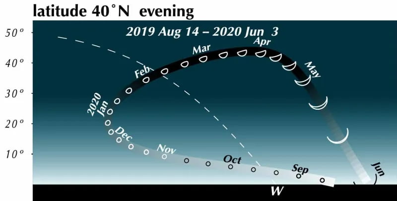
Things are different with theories of celestial motion, where people definitely disagreed. The basic empirical data concerns how bright spots move across the sky. First of all, there is the sun, moving east to west every day. But also the moon, and lots of other bright little spots. Most of those move together, but some take their own curious paths: Jupiter, Mars, Venus, and their ilk (see the path of Venus below). For example, bodies like Mars sometimes move in a kind of back-and-forth swipe across the sky (given a fixed vantage point on Earth), called retrograde, see the animation below. For theories of celestial motion, that’s the basic kind of data we want our models to capture: Paths that spots take across the sky.
Our current theories for capturing this basic data derive the easily observable (paths that bright spots take across the sky) from the much harder to observe (bodies pulling each other around out there in space). These days, we capture this data with a heliocentric model (sun in center), and planets on elliptical orbits around it. The movement of the bright dots is more or less a projection from the actual 3D movement in space onto the 2D-ish sky. Maybe we were taught in middle school that people used to believe that the earth was at the center (geocentric models), just because they saw the sun move across the sky, and because humans are all a bit narcissistic.
Now, if that’s the degree of familiarity you have with the history of astronomy, it may come as a surprise to you that the ancient geocentric model of Ptolemy (c. 100-170) is both sophisticated, and quite good at actually describing/predicting those paths. The key aspects are: a) an earth that is slightly off-center, and b) the possibility for bodies like Venus and Mars to move not in a circle, but in an epicycle: A small circular motion around the circle (see Mars’ looping orbit in the gif below).
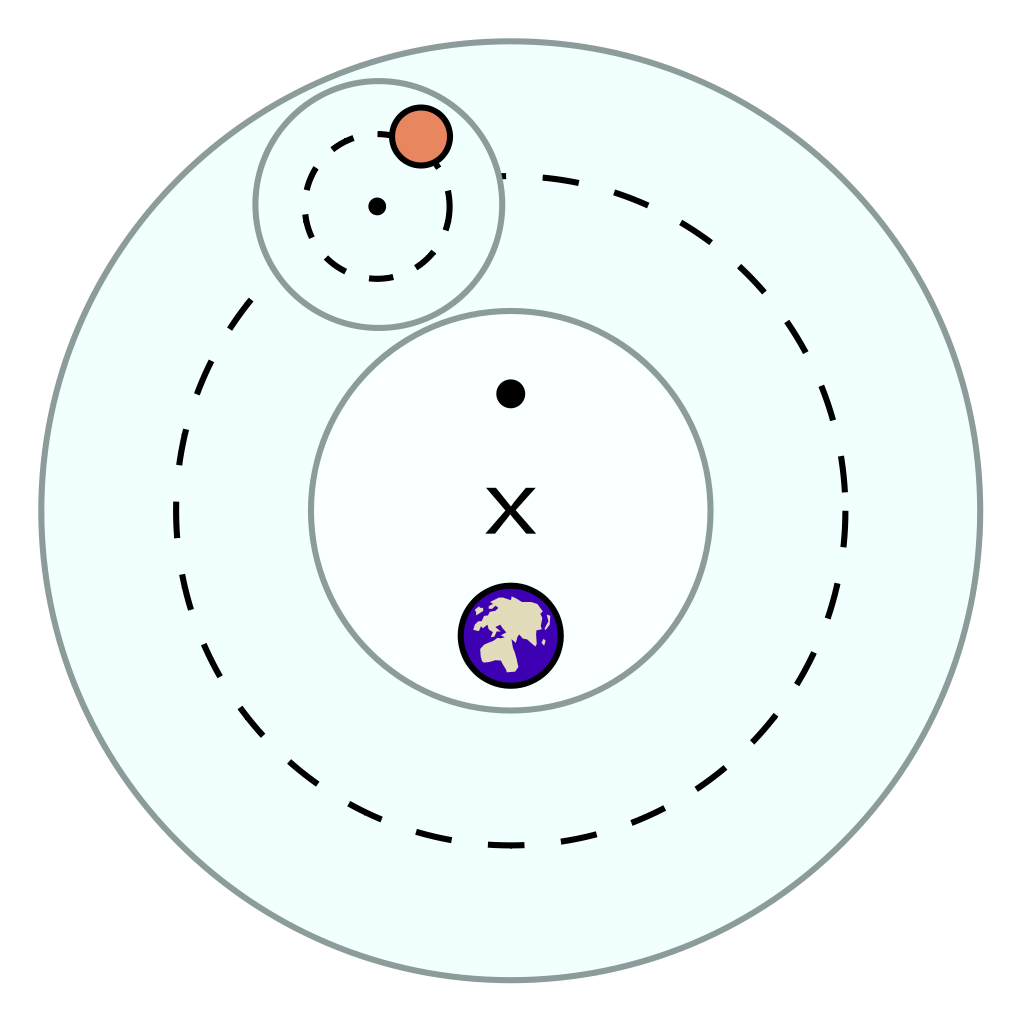
Epicycles derive facts about the path of bright spots in the sky – we can see Mars in retrograde in the animation above: Effectively, the hypothesis is that Mars doesn’t directly orbit Earth, it actually orbits a point that orbits Earth, i.e., two circular movements. Sometimes the sum of these two movement cycles will mean Mars goes “backwards”, and thus the sum of two simple aspects (circular movement) gives us the complex facts about a loopy movement path in the sky.
Anyways – if you want to learn more about the actual history of astronomy (as opposed to the weird middle school version we all had to learn), we recommend this series of blog posts by scifi author Michael Flynn (there might be the occasional quarrel after all, whoops!). What’s important for us here, is that the heliocentric models that we all learn about now… weren’t really any better at accounting for those paths of little (or big) bright spots in the sky than their geocentric Ptolemaic competition. As far as the immediately observable data was concerned, the models were, well, pretty much equivalent. One might even say they were the astronomy version of “weakly equivalent”.
Why do we now scoff at geocentric theories and believe heliocentric ones when they both adequately captured the observed paths of celestial bodies? What changed the game? The answer is a new kind of data: the phases of Venus. While both geocentric and heliocentric theories could account for the original data about the paths of bright spots, it turns out that only the heliocentric theories could account for the crescent shapes of those bright spots.
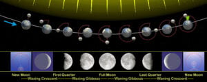
Well, everyone knew the moon had phases. It’s pretty obvious, even to us moderns, that the moon waxes and wanes. When better telescopes arrived, people took a closer look at some of those moving bright spots, and found out that other celestial bodies also have phases. Essentially, phases arise from the relative positions of three bodies: The earth (the vantage point), the sun (the light source), and the third body (the moon, Venus, etc): Only one side of a celestial body gets sunshine at any given moment (it’s “day time” over there), but that’s not necessarily the same part that is facing our way. Instead, we might see some part of the body where it’s day, and some part where it’s night. (The same is true the other way around, of course – check out the phases of the earth from the moon, though I guess they couldn’t see that stuff back then). The following figure shows how this works (in a heliocentric model) to make the moon wax and wane.
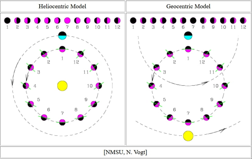
Both models apparently did pretty well for the moon in this regard. But for Venus, they made completely different predictions (see below). Both geocentric and heliocentric models postulated an “underlying structure” for space that could not be observed directly (no artificial satellites that could take pictures of a pale blue dot yet, the only perspective anybody had was that from earth). The structures of space that these models postulated were abstractions, useful in deriving the observable data: We could observe the angle between the sun and Venus in the sky, but not their actual distances from Earth (since the depth information is lost in projection – recall that our observations are 2-dimensional, but both geocentric and heliocentric models are 3-dimensional).
Now, once the movement paths were stipulated in a way that could account for the initial observations (movement of spots across the sky), one could predict the relative positions of the sun, Earth, and Venus. Hence, one could calculate the angle between the daylight area of Venus, and the area that was facing earth: The models predicted different phases of Venus to correlate with different movements of the bright spot with that name across the sky.
If you want to see an animated version, there’s a lovely visualization for each model right here:
Venus Phases in the Heliocentric Model
Venus Phases in the Ptolemaic Geocentric Model
To sum up, before we finally return to linguistics: Both models made assumptions about the way bodies move in the heavens (unobservable at the time). Both models could derive the movements of bodies in the sky (observable) as a projection from one onto the other. Both models also made predictions about the phases of celestial bodies, again based on the same assumptions about orbits. But only for one model were these predictions actually in line with the newly observable data, the phases of Venus. This was the new kind of data that made the heliocentric models win out (there’s more stuff, but this isn’t an astronomy post… arguably). Of course, centuries later, we actually launched artificial satellites, thus giving us “3D vision in the heavens”, which allowed us to more directly observe the formerly unobservable movements, but even before that, the set of abstractions from one theory did better than the other.
Now, we may say that two models for the movement of celestial bodies are weakly equivalent if they generate the same movement of bright spots across the sky (2D). But only if they were to also assign them the same movement in the heavens (3D) would we call them strongly equivalent. Astronomers, it turns out, did not care whether geocentric models are weakly equivalent to heliocentric ones. They cared about which one covered the larger range of relevant phenomena.
This means that equivalency (weak or strong) can only be understood as relative to a particular collection of phenomena (i.e., relative to the data that the theory is here to explain). In short, it is scientifically ridiculous to focus on the fact that geocentric theories are weakly equivalent to heliocentric ones relative to predicting the paths of bright spots across the sky. Clearly, that’s not the only desideratum, and it is rather blinkered to get stuck worrying about only one particular type of data. The astronomers of the day knew this, even though nobody could directly observe any movement in the heavens – at that point a purely theoretical, abstract postulate.
Syntacticians are, unfortunately, in a position reminiscent of the one that 16th century astronomers found themselves in (possibly worse, but probably with less persecution): Just as astronomers postulated unobservable movement in the heavens to explain observable movement in the sky, syntacticians postulate unobservable phrasal nodes (say, a verb phrase in English) to account for the things we directly observe: Strings such as “Jo kicked the prof” or “Mary had them eat a cake” and their associated meanings. To a syntactician, strings are a little like the bright spots moving across the sky: They are the most immediately observable phenomenon we have. We certainly want to explain them. Like the astronomers, though, we too keep uncovering new phenomena, and we definitely care about whether our previous unobservables (our abstract postulates, our structure of phrasal nodes) can account for all of them. Back to weak equivalence: Two models are weakly equivalent (relative to strings) if they generate the same set of them, even when they do so with different structures. For the purpose of this particular empirical domain – the set of possible strings – two models may well be indistinguishable. As with astronomy, the real test is whether phrasal nodes (the abstract objects that we use to derive our strings) are also useful for other kinds of data. The answer is obviously yes. Just like astronomers don’t just work only on the movement of bright spots in the sky anymore, syntacticians aren’t just (or even primarily) concerned with strings. In what follows, we will highlight some additional kinds of data that syntacticians care about, and show that all of them can be (at least mostly) handled using the abstractions that can also derive strings.
For instance, we know full well that a single string can actually correspond to multiple meanings. Take the standard example from day 1 of a Ling 101 class in (1), which exhibits a classic ambiguity:
(1) The Martian saw the frog with the telescope.
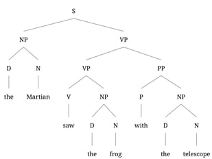
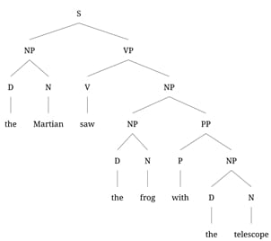
Either the Martian has the telescope, and uses it to see the frog, or the frog has the telescope, and the Martian sees that frog. That such ambiguities exist is relevant to linguists in exactly the same way that the phases of Venus were to astronomers: We want them to follow from the same abstract syntactic structure that we used to generate the string. We generally introduce this idea to new linguistics students with toy phrase structure grammars like the one in (2):
This grammar has two ways of producing the string in (1), namely those in (3):
By hypothesis, these two parses correspond to the two meanings: The PP modifies either the seeing event, as an instrument, in which case it is the sister of VP. Or it modifies the frog, in which case it is the sister of NP.
Why do linguists think some hypothesis along these lines is on the right track? Because the NP nodes – our “orbits”, which we cannot observe directly – not only give us the two meanings, but they also let us account for a host of other properties. Take instance, passive sentences. We might describe some aspect of the relation between an active and a passive sentence by saying that the NP that is the sister of the verb in the active sentence is the subject of the sentence in the passive (or, in our analysis, the sister of VP), and the subject of the active sentence is the argument of a by PP in the passive. Now, in one case, the object is the frog, and in the other it is the frog with the telescope. So, if we make a passive sentence out of the active sentences above, we expect them to be disambiguated, because the two structures do no longer map onto the same string. In particular, (4b) does not have the reading where the telescope is used for seeing the frog.
The grammar in (2) allows us to capture this ambiguity and its disappearance under passivization. In entirely parallel fashion, we could look at another property associated with the NP node: Pronominalization. Maximal NP nodes can be replaced by pronouns such as they, it, she, he. Now, let’s take a look at (5), in which we “pronominalized” the NP ‘the frog’ from (3a). Again, the ambiguity disappears. This fact follows from the particular phrase structures we used to generate the string and not from the string itself.
(5) The Martian saw it with the telescope.
If the phrasal nodes are like the orbits, then structural ambiguities, passivization and pronominalization are like the phases of Venus: Properties that should follow from the same assumptions that generated the strings.
Now, let’s take an alternative grammar G’ that lacks the clause (2-b-v), the verb phrase modification VP -> VP PP. Such a grammar is weakly equivalent to G; both grammars generate exactly the same set of strings, which we can characterize as in (6).
(6) D N (PP*) V D N (PP*)
Despite their weak equivalence, linguists will obviously reject G’ in favor of G. Just as the heliocentric and the geocentric models couldn’t be distinguished solely on the basis of the movement in the sky, G and G’ cannot be distinguished solely on the basis of the set of strings they characterize. But just like the geocentric model failed to offer an adequate account of the phases of Venus, G’ fails to offer an account of the ambiguity we observed – it lacks the ability to generate two different structures corresponding to a single string. It doesn’t make the right nodes, the right structural relations available to account for all the other phenomena linguists care about. Here’s a list (highly abridged) of some other aspects of grammar that syntacticians worry about, and all of them have been argued to depend on structural relations that the phrase structure makes available.
- Scope: A girl saw every cat. (is there one girl or more than one?)
- Binding: Maryi said that shei/j came.
- Agreement: The girls from the story are/*is generating phrase structures.
- Case: He/*him came. (maybe could do a string-based theory for English, but not for more complicated case languages – see Marantz 1991, Baker 2015)
- Islands for movement: That John went home is likely v. *Who is that ___ went home likely? (Ross 1967 p.86)
- Ellipsis licensing: Valentine is a good volleyball player and I heard a rumor that Alexander is [a good volleyball player] too. v. *Valentine is a better volleyball player than I heard a rumor that Alexander is [a good volleyball player] too. Stolen from Max Papillon’s tweet
- Long Distance dependencies like “if…then”, “either…or” (Chomsky ‘57 p 22)
(See also section 2 of Adger & Svenonius 2015, they make a related point with related examples.)
In conclusion, what we really care about is whether an abstraction such as phrase structure can tie together these various phenomena. It’s for this reason that we care (a lot) about all those non-terminal nodes that, say, a phrase structure grammar generates. The ones that weak equivalence doesn’t pertain to. The pesky theoretical abstractions that aren’t (directly) observable have turned out to be the most useful tool in our box so far, both for analyzing and for discovering all these other phenomena – that’s why it’s still true that “we have no interest, ultimately, in grammars that generate a natural language correctly but fail to generate the correct set of structural descriptions” – Chomsky & Miller (1963:297).
Memorized vs. Computed
I have previously written about why I believe that distinctions in the literature between words (or sentences) that are “stored” as units vs. words (or sentences) that are “computed” are not well articulated. I claimed, instead, that, in a sense that is crucial for understanding language processing, all words (and all sentences) are both stored AND computed, even those words and sentences a speaker has never encountered before. A speaker stores or memorizes all the infinite number of words (and sentences) in his/her language by learning a grammar for the language. Attempts in the literature to distinguish the stored words from the computed ones fail to be clear about what it means to store or compute a word – particularly on what it means to memorize a word. I claimed that, as we become clear on how grammars can be used to recognize and produce words (and sentences), any strict separation between the stored and the computed disappears.
Despite my earlier efforts, however, I find that I have not convinced my audience. So here I’ll follow a line of argument suggested to me by Dave Embick and try again.
Let’s start with Jabberwocky, by Lewis Carroll of course (1871, this text from Wikipedia):
Twas brillig, and the slithy toves
Did gyre and gimble in the wabe;
All mimsy were the borogoves,
And the mome raths outgrabe.
“Beware the Jabberwock, my son!
The jaws that bite, the claws that catch!
Beware the Jubjub bird, and shun
The frumious Bandersnatch!”
He took his vorpal sword in hand:
Long time the manxome foe he sought—
So rested he by the Tumtum tree,
And stood awhile in thought.
And as in uffish thought he stood,
The Jabberwock, with eyes of flame,
Came whiffling through the tulgey wood,
And burbled as it came!
One, two! One, two! And through and through
The vorpal blade went snicker-snack!
He left it dead, and with its head
He went galumphing back.
“And hast thou slain the Jabberwock?
Come to my arms, my beamish boy!
O frabjous day! Callooh! Callay!”
He chortled in his joy.
‘Twas brillig, and the slithy toves
Did gyre and gimble in the wabe;
All mimsy were the borogoves,
And the mome raths outgrabe.
The poem is full of words that the reader might not recognize and/or be able to define. Quick quiz: which words did Carroll make up?
Not so easy, at least for me. Some words that Carroll was the first to use (as far as lexicographers know) have entered the language subsequently, e.g., vorpal (sword). What about chortle? Are you sure? How about gyre? Gimble? Beamish? Whiffling?
The fact is that when we encounter a word in context, we use our knowledge of grammar, including our knowledge of generalizations about sound/meaning connections, to assign a syntax and semantics to the word. (Chuang, Yu-Ying, et al. “The processing of pseudoword form and meaning in production and comprehension: A computational modeling approach using linear discriminative learning.” Behavior research methods (2020): 1-32.) Suppose the word is one we have not previously encountered, but it is already in use in the language. Can we tell it’s a “real” word as opposed to Jabberwocky? That the word has found a place in the language probably means that it fits with generalizations in the language, including those about correlations between sound and meaning and between sound and syntactic category. Children must be in this first encounter position all the time when they’re listening – and I doubt that many of them are constantly asking, is that really a word of English? Suppose, now, that the-new-to-us word in question is actually not yet a word in use in English, as was the case for the first readers of Jabberwocky encountering chortle. In the course of things, there’s no difference between encountering in context a word that’s in use and you haven’t heard yet, but fits the grammar of your language, and one that the speaker made up, but also fits the grammar of your language equally well. Lewis Carroll made up great words, extremely consistent with English, and many of them stuck.
Speakers of English have internalized a phonological grammar (a phonology) that stores our knowledge of the well-formedness of potentially infinite strings of phonemes. The phonotactics of a language include an inventory of sounds (say an inventory of phonemes) and the principles of phonotactics – the sounds’ legal combinations. The phonology – the phonotactic grammar – stores (and generates) all the potential words of the language, but doesn’t distinguish possible from “actual” words by itself. Are the “actual” words distinguished as phoneme-strings carrying the extra feature [+Lexical Insertion], as Morris Halle once claimed for morphologically complex words that are in use as opposed to potential but not “actual” words (Halle, M. (1973). Prolegomena to a theory of word formation. Linguistic inquiry, 4(1), 3-16)? It’s not particularly pertinent to the question at hand whether people can say, given a string of letters or phonemes in isolation, this a word of my language. Experimental subjects are asked to do this all the time in lexical decision experiments, and some are surprisingly accurate, as measured against unabridged dictionaries or large corpora. Most subjects are not so accurate, however, as one can see from examining the English Lexicon Project’s database of lexical decisions – 85% correct is fairly good for both the words (correct response is yes) and pronounceable non-words (correct response is no) in that database. Lexical Decision is a game probing recognition memory – can I recover enough of my experiences with a letter or phoneme string to say with some confidence that I encountered it before in a sentence? A better probe of our knowledge of potential and actual words is placing the strings in sentential context – the Jabberwocky probe. Do we think a Jabberwocky word is a word in our language. Here we see that our judgments are graded, with no clear intuition corresponding to a binary word/non-word classification.
For phonology, it’s somewhat clear what we mean when we say that the generative grammar “stores” the forms of potential and existing words in the language. The consequences of this for the Chomskyan linguist (committed to the principle that there are not separate competence and performance grammars) is that the phonological grammar is used in recognizing and producing the words. For committed Chomskyans, like me, at a first pass, we expect that phonotactic well-formedness will always play a role in word recognition and production – “knowing” a word doesn’t exempt it from obligatory “decomposition” via the grammar in use into, e.g., phonemes, and analysis via the phonotactic grammar. “Retrieving” the phonological form of a word from memory and “generating” it from the grammar become the same process.
What is, then, the difference between words like chatter and Jabberwocky like chortle? Although our grammar will assign a meaning to any well-formed possible word, without sentential or other context, the meaning might be vague. As we experience words in context, we can develop sharper accounts of their meaning, perhaps primarily via word co-occurrences. The sharpness of a semantic representation isn’t a property of the phonological grammar, but it is a property of the grammar as a whole. For linguists, a “whole” grammar includes, in addition to a syntax that organizes morphemes into hierarchical tree structures and a phonology that maps the syntactic structure into a structured sequence of prosodic units like phonological words, also what Chomsky calls a language’s “externalization” in the conceptual system, i.e., in this case the meaning of words.
In important ways, words are like human faces to human speakers. We have internalized a grammar of faces that allow us to recognize actual and potential faces. We store this grammar, at least partially, in what is called the Fusiform Face Area. Recognizing faces (as faces) involves obligatory decomposition into the elements of a face (like the eyes, ears, and nose) whose grammatical combinations the face grammar describes. For faces, we don’t call the faces of people that we haven’t seen “potential” or “pseudo” faces – they’re just faces, and the faces of people that we have encountered (and can recall as belonging to people we’ve seen or met) we call “familiar” faces. For words, I propose we adopt the same nomenclature – words and potential words should just be “words,” while words to which we push the “yes” button to in Lexical Decision experiments should be called “familiar words.”
Note that, for written words, there’s an even greater parallel between words and faces. Our orthographic grammar, describing the orthotactics of the language, generates thus stores all the orthographic forms of the words of the language. From neuroscientific studies, we know that the orthographic grammar – and thus the orthographic forms of words – is (at least partially) stored in an area of the brain adjacent to the Fusiform Face Area (called the “Visual Word Form Area”), and the recognition of words follows a parallel processing stream and time frame as the recognition of faces. One can speculate (as I will in a future post) that the phonological grammar and thus the phonological forms of words (really morphemes of course) live in secondary auditory cortices on the superior temporal lobe, where auditory word recognition is parallel to the recognition of faces and visual word forms, with the interesting complication that the recognition process plays out over time, as the word is pronounced.
[To be continued…..]
© 2024 NYU MorphLab
Theme by Anders Noren — Up ↑