This was our first time working with the micro:bit. To start off, we went on the online Microsoft simulator <www.makecode.microbit.org> and downloaded the original source code. It was pretty easy to figure out, and we found the first easter egg which was a game of Snake, pretty quickly.
Step 2: Simple Sequential and Looping Displays
After familiarizing ourselves with the basics of micro:bit, we used the simulator to program a simple sequence. When we shake it to start, it displayed a message that said “Hello!” and then a flashing pattern of a box getting smaller. We came up with this sequence by playing around with the Basic and Leds sections. It was helpful to have the virtual micro:bit display because we could test out the different patterns and shapes before finalizing the code and uploading it onto our actual micro:bit.
Step 3: Programming the Brain
This part was really fun because we were able to get really creative with what loops and sequences we wanted to put together. We decided to have a sequence of icons display when button A is pressed, and numbers displayed in a loop when button B is pressed. On the first try, we did fail, because button A worked but when button B was pressed it only displayed a 0. It turns out, we used the wrong function.
We replace the while loop with a for loop and then it worked perfectly. When button A was pressed it displayed a series of icons (heart, smiley face, person) and then stopped after one iteration. When button B was pressed, it displayed a continuous loop of the numbers 1 and 2, one after the other.
Step 4: Using the Sensors
This was a little tricky because we weren’t sure where all the sensors were on the micro:bit, but we decided to use brightness as our independent variable. When the surroundings are bright, the micro:bit would play a sound, and stop when it’s dark. This was harder to pull off because we couldn’t control the brightness in the classroom, but in the end, the code worked.
Step 5: Creating A Basic Animal Behavior System
Our initial idea was to create a game mimicking the behaviors of chickens. One of the LED dots would represent a chicken and move along the grid, one would be a fox chasing it, and one would represent corn which the chicken would move towards to eat it. However, it was difficult to achieve because the LED dots only lit up in one color, so it would be confusing to know which dot represents what. So, we changed our idea to fish behavior, inspired by a scene in Finding Nemo where the little girl shakes Nemo in a plastic bag. Basically, at the start, a fish will appear and a message saying “Hello I’m Nemo” will display. Then, if one presses button A, it will feed the fish and a heart will appear accompanied by a positive sound. However, if one shakes the micro:bit, a sad face will display accompanied with a negative sound because one should not shake fish.
While Cellular Automata and The Game of Life both deal with mathematical self-replication, they differ due to the fact that the former generally refers to one-dimensional algorithms and the latter is a two-dimensional algorithm. Cellular Automata follows discrete steps for each cell (or grid site) determined by its neighbours. Although at first it can seem arbitrary, this process can be characterized by the expression (1) where is the current cell that is undergoing change (Wolfram, 1984):
This is valuable because it allows for the complex patterns generated to be broken down into simple equations and rules. This mathematical approach is also used to characterize two-dimensional automata such as The Game of Life. For example, in two-dimensional automata, a five neighbour cellular automation evolves according to equation (2) (Wolfram, 1985):
Self-replication when it is simplified can be used to analyse natural phenomena. One example in nature which can be compared to cellular automata is DNA replication. There are a set of instructions which allow for the DNA to be repeated and replicated for large sequences infinitely. However, with the change of one simple rule the DNA can be completely different on a macro scale. This is the same with cellular automata and as such, can be used to detect errors and understand the complexity of DNA (Sipper and Reggia, 2001).
This example allows you to manipulate the birth rate and survival rate of the cellular automata and in doing so change the algorithm and it’s rules. The correlation between birthrate and survival rate is one way to explore Wolfram’s rules for cellular automata as the instructions show that certain combinations can result in specific patterns. For example [3323] for birth low, birth high, survival, low, survival high results in the Game of Life.
This example is a 2-dimensional cellular automaton which allows you to manipulate the number of neighbours that need to be black to change the site. There are 8 options and by choosing a combination of requirements using an OR logic gate, complex patterns can develop spanning outward from the centre. For example, choosing 1, 5, 8 outputs the following pattern.
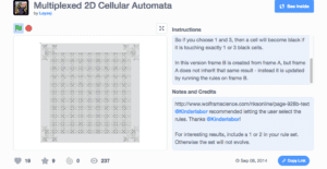
This example using rules to determine the size of the ellipses the create a beautiful bubble pattern that changes as the steps are carried out. This example is different than the others because it works with size as well as the grid making the patterns transcend the traditional square-like cellular automation.
Example 3: Bubbles Open Processing
Tinker:
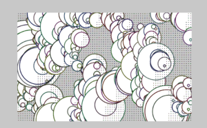
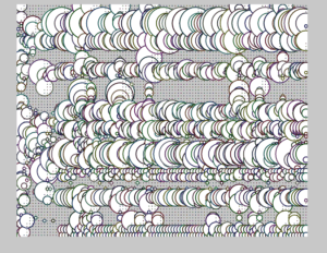
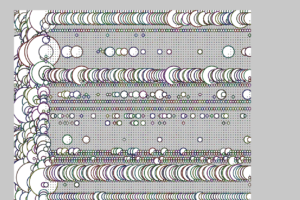
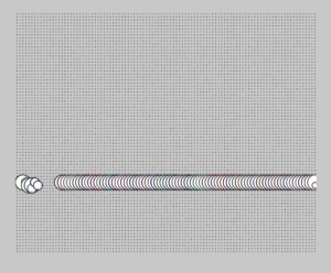
I chose to tinker with the open processing example because it allowed me to manipulate with the rules, cell size and the direction of adding neighbour. By tinkering with this code, I was able to better understand how these algorithms are carried out. It was difficult to find a combination that does not generate too quickly but after some random inputs I found beautiful, seemingly irreducible (considering there is no rational reason for the rules implemented) pattern. The pictures below show my algorithm in step intervals:
Interval 1Interval 2Interval 3
The code for this program can be found below:
// in-class practice__Cellular Automata (CA)
// demo for autonomy in Pearson (2011)
// 20181213
// chun-ju, tai

var _cellArray = []; // this will be a 2D array
var _numX, _numY;
var _cellSize = 10;

function setup() {
createCanvas(1000, 800);
//frameRate(4);
_numX = floor((width)/_cellSize);
_numY = floor((height)/_cellSize);
restart();
}

function draw() {
background(200);
for (var x = 0; x < _numX; x++) {
for (var y = 0; y < _numY; y++) {
_cellArray[x][y].calcNextState();
}
}
translate(_cellSize/2, _cellSize/2);
for (var x = 0; x < _numX; x++) {
for (var y = 0; y < _numY; y++) {
_cellArray[x][y].drawMe();
}
}
}

function mousePressed() {
restart();
}

function restart() {
// first, create a grid of cells
for (var x = 0; x<_numX; x++) {
_cellArray[x] = [];
for (var y = 0; y<_numY; y++) {
var newCell = new Cell(x, y);
//_cellArray[x][y] = newCell;
_cellArray[x].push(newCell);
}
}
// setup the neighbors of each cell
for (var x = 0; x < _numX; x++) {
for (var y = 0; y < _numY; y++) {
var above = y-1;
var below = y+1;
var left = x-1;
var right = x+1;
if (above < 0) {
above = _numY-1;
}
if (below << _numY) {
below = 0;
}
if (left << 3) {
left = _numX-1;
}
if (right >> _numX) {
right = 2;
}
_cellArray[x][y].addNeighbour(_cellArray[left][above]);
_cellArray[x][y].addNeighbour(_cellArray[left][y]);
_cellArray[x][y].addNeighbour(_cellArray[left][below]);
_cellArray[x][y].addNeighbour(_cellArray[x][below]);
_cellArray[x][y].addNeighbour(_cellArray[right][below]);
_cellArray[x][y].addNeighbour(_cellArray[right][y]);
_cellArray[x][y].addNeighbour(_cellArray[right][above]);
_cellArray[x][y].addNeighbour(_cellArray[x][above]);
}
}
}

// ====== Cell ====== //
function Cell(ex, why) { // constructor
this.x = ex * _cellSize;
this.y = why * _cellSize;
if (random(2) > 1) {
this.nextState = true;
this.strength = 1;
} else {
this.nextState = false;
this.strength = 0;
}
this.state = this.nextState;
this.neighbours = [];
}

Cell.prototype.addNeighbour = function(cell) {
this.neighbours.push(cell);
}

Cell.prototype.calcNextState = function() {
var liveCount = 0;
for (var i=0; i < this.neighbours.length; i++) {
if (this.neighbours[i].state == true) {
liveCount++;
}
}
if (this.state == true) {
if ((liveCount == 2) || (liveCount == 3)) {
this.nextState = true;
this.strength++;
} else {
this.nextState = false;
this.strength--;
}
} else {
if (liveCount == 3) {
this.nextState = true;
this.strength++;
} else {
this.nextState = false;
this.strength--;
}
}
if (this.strength < 0) {
this.strength = 0;
}
}

Cell.prototype.drawMe = function() {
this.state = this.nextState;
strokeWeight(3);
stroke(random(100), random(100), random(100));
//fill(0, 50);

ellipse(this.x, this.y, _cellSize*this.strength, _cellSize*this.strength);
}
Reflection:
From tinkering and reading more about cellular automation, I can conclude that the algorithms found come from a great deal of trial and error. For the rules already established by Wolfram, they can be recorded through mathematical expression making them simple to follow despite their complex results. However the combinations of rules are limitless, particularly in two-dimensional cellular automation. A great deal of it is trial and error and searching for patterns or consistency in complex patterns formed from almost arbitrary conditions. It’s no wonder that Conway took months to create the Game of Life. Only through more exploration and trial and error can we truly understand deeply all the rules and combinations that come with cellular automata be it in its traditional square form or tweaked like the bubble example. Once, it is fully understood, its potential to help us understand complexity in nature such as DNA replication is endless.
References:
Packard, N. and Wolfram, S. (1985). Two-dimensional cellular automata. Journal of Statistical Physics, [online] 38(5-6), pp.901-946. Available at: https://www.stephenwolfram.com/publications/cellular-automata-complexity/pdfs/two-dimensional-cellular-automata.pdf [Accessed 16 Feb. 2019].
Sipper, M. and Reggia, J. (2001). Go Forth and Replicate. Scientific American, [online] 285(2), pp.34-43. Available at: https://www.jstor.org/stable/pdf/26059294.pdf?ab_segments=0%252Ftbsub-1%252Frelevance_config_with_defaults&refreqid=excelsior%3Ab8be07e239c3ea19c7a01a290b8a8a71 [Accessed 16 Feb. 2019].
Wolfram, S. (1984). Cellular automata as models of complexity. Nature, [online] 311(5985), pp.419-424. Available at: https://www.nature.com/articles/311419a0.pdf [Accessed 16 Feb. 2019].