Lab Report #1: Cellular Automata

Research:

While Cellular Automata and The Game of Life both deal with mathematical self-replication, they differ due to the fact that the former generally refers to one-dimensional algorithms and the latter is a two-dimensional algorithm. Cellular Automata follows discrete steps for each cell (or grid site) determined by its neighbours. Although at first it can seem arbitrary, this process can be characterized by the expression (1) where  is the current cell that is undergoing change (Wolfram, 1984):

(1)   a_i^(t+1)= ∅[a_(i-r)^((t)),a_(i-r+1)^((t))…a_(i+r)^((t)) ]    

This is valuable because it allows for the complex patterns generated to be broken down into simple equations and rules. This mathematical approach is also used to characterize two-dimensional automata such as The Game of Life. For example, in two-dimensional automata, a five neighbour cellular automation evolves according to equation (2) (Wolfram, 1985):  

(2)   a_(i,j)^(t+1)= ∅[a_(i,j)^((t)),a_(i,j+1)^((t)),a_(i+1,j)^((t)),a_(i,j-1)^((t)),a_(i-1,j)^((t)) ]

Self-replication when it is simplified can be used to analyse natural phenomena. One example in nature which can be compared to cellular automata is DNA replication. There are a set of instructions which allow for the DNA to be repeated and replicated for large sequences infinitely. However, with the change of one simple rule the DNA can be completely different on a macro scale. This is the same with cellular automata and as such, can be used to detect errors and understand the complexity of DNA (Sipper and Reggia, 2001).

Code Examples:

Example One: Birthrate

https://scratch.mit.edu/projects/10100662/

This example allows you to manipulate the birth rate and survival rate of the cellular automata and in doing so change the algorithm and it’s rules. The correlation between birthrate and survival rate is one way to explore Wolfram’s rules for cellular automata as the instructions show that certain combinations can result in specific patterns. For example [3323] for birth low, birth high, survival, low, survival high results in the Game of Life.

Example 1: Birthrate

Example Two: Two Dimensional Nearest Neighbour

https://scratch.mit.edu/projects/26321491/

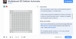
This example is a 2-dimensional cellular automaton which allows you to manipulate the number of neighbours that need to be black to change the site. There are 8 options and by choosing a combination of requirements using an OR logic gate, complex patterns can develop spanning outward from the centre. For example, choosing 1, 5, 8 outputs the following pattern.
2D Automata
Example 2: 2D Automata

Example Three: OpenProcessing Bubble Manipulation

https://www.openprocessing.org/sketch/644405

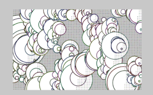
This example using rules to determine the size of the ellipses the create a beautiful bubble pattern that changes as the steps are carried out. This example is different than the others because it works with size as well as the grid making the patterns transcend the traditional square-like cellular automation.
Example 3: Bubbles Open Processing

Tinker:

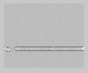
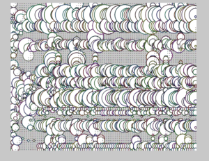
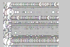
I chose to tinker with the open processing example because it allowed me to manipulate with the rules, cell size and the direction of adding neighbour. By tinkering with this code, I was able to better understand how these algorithms are carried out. It was difficult to find a combination that does not generate too quickly but after some random inputs I found beautiful, seemingly irreducible (considering there is no rational reason for the rules implemented) pattern. The pictures below show my algorithm in step intervals:
Interval 1: Full bubbles
Interval 1
Interval 2: Changed pattern
Interval 2
Interval 3: One row of bubbles
Interval 3

The code for this program can be found below:

// in-class practice__Cellular Automata (CA) 
// demo for autonomy in Pearson (2011)
// 20181213
// chun-ju, tai

var _cellArray = []; // this will be a 2D array
var _numX, _numY;
var _cellSize = 10;

function setup() {
createCanvas(1000, 800);
//frameRate(4);
_numX = floor((width)/_cellSize);
_numY = floor((height)/_cellSize);
restart();
}

function draw() {
background(200);
for (var x = 0; x < _numX; x++) {
for (var y = 0; y < _numY; y++) {
_cellArray[x][y].calcNextState();
}
}
translate(_cellSize/2, _cellSize/2);
for (var x = 0; x < _numX; x++) {
for (var y = 0; y < _numY; y++) {
_cellArray[x][y].drawMe();
}
}
}

function mousePressed() {
restart();
}

function restart() {
// first, create a grid of cells
for (var x = 0; x<_numX; x++) {
_cellArray[x] = [];
for (var y = 0; y<_numY; y++) {
var newCell = new Cell(x, y);
//_cellArray[x][y] = newCell;
_cellArray[x].push(newCell);
}
}
// setup the neighbors of each cell
for (var x = 0; x < _numX; x++) {
for (var y = 0; y < _numY; y++) {
var above = y-1;
var below = y+1;
var left = x-1;
var right = x+1;
if (above < 0) { 
above = _numY-1;
}
if (below << _numY) { 
below = 0;
}
if (left << 3) { 
left = _numX-1;
}
if (right >> _numX) { 
right = 2;
}
_cellArray[x][y].addNeighbour(_cellArray[left][above]);
_cellArray[x][y].addNeighbour(_cellArray[left][y]);
_cellArray[x][y].addNeighbour(_cellArray[left][below]);
_cellArray[x][y].addNeighbour(_cellArray[x][below]);
_cellArray[x][y].addNeighbour(_cellArray[right][below]);
_cellArray[x][y].addNeighbour(_cellArray[right][y]);
_cellArray[x][y].addNeighbour(_cellArray[right][above]);
_cellArray[x][y].addNeighbour(_cellArray[x][above]);
}
}
}

// ====== Cell ====== //
function Cell(ex, why) { // constructor
this.x = ex * _cellSize;
this.y = why * _cellSize;
if (random(2) > 1) {
this.nextState = true;
this.strength = 1;
} else {
this.nextState = false;
this.strength = 0;
}
this.state = this.nextState;
this.neighbours = [];
}

Cell.prototype.addNeighbour = function(cell) {
this.neighbours.push(cell);
}

Cell.prototype.calcNextState = function() {
var liveCount = 0;
for (var i=0; i < this.neighbours.length; i++) {
if (this.neighbours[i].state == true) {
liveCount++;
}
}
if (this.state == true) {
if ((liveCount == 2) || (liveCount == 3)) {
this.nextState = true;
this.strength++;
} else {
this.nextState = false;
this.strength--;
}
} else {
if (liveCount == 3) {
this.nextState = true;
this.strength++;
} else {
this.nextState = false;
this.strength--;
}
}
if (this.strength < 0) {
this.strength = 0;
}
}

Cell.prototype.drawMe = function() {
this.state = this.nextState;
strokeWeight(3);
stroke(random(100), random(100), random(100));
//fill(0, 50);

ellipse(this.x, this.y, _cellSize*this.strength, _cellSize*this.strength);
}

Reflection:

From tinkering and reading more about cellular automation, I can conclude that the algorithms found come from a great deal of trial and error. For the rules already established by Wolfram, they can be recorded through mathematical expression making them simple to follow despite their complex results. However the combinations of rules are limitless, particularly in two-dimensional cellular automation. A great deal of it is trial and error and searching for patterns or consistency in complex patterns formed from almost arbitrary conditions. It’s no wonder that Conway took months to create the Game of Life. Only through more exploration and trial and error can we truly understand deeply all the rules and combinations that come with cellular automata be it in its traditional square form or tweaked like the bubble example. Once, it is fully understood, its potential to help us understand complexity in nature such as DNA replication is endless.

References:

Packard, N. and Wolfram, S. (1985). Two-dimensional cellular automata. Journal of Statistical Physics, [online] 38(5-6), pp.901-946. Available at: https://www.stephenwolfram.com/publications/cellular-automata-complexity/pdfs/two-dimensional-cellular-automata.pdf [Accessed 16 Feb. 2019].

Sipper, M. and Reggia, J. (2001). Go Forth and Replicate. Scientific American, [online] 285(2), pp.34-43. Available at: https://www.jstor.org/stable/pdf/26059294.pdf?ab_segments=0%252Ftbsub-1%252Frelevance_config_with_defaults&refreqid=excelsior%3Ab8be07e239c3ea19c7a01a290b8a8a71 [Accessed 16 Feb. 2019].

Wolfram, S. (1984). Cellular automata as models of complexity. Nature, [online] 311(5985), pp.419-424. Available at: https://www.nature.com/articles/311419a0.pdf [Accessed 16 Feb. 2019].
Bio | Week 1 | Lab Report: Cellular Automaton(Terrence Tu)

      As far as we learned from the class, we were still talking about cellular automaton below two dimensions. Conway’s Life of Game is a kind of two-dimensional cellular automation while Wolfram’s “The Crucial Experiment” of A New Kind of Science is doing one-dimensional cellular automaton and representing the its behavior in two-dimensional graph. From both of the cases, we can that significant complexity occurs from very simple programs.

      From my perspective, however, considering of the three-dimensional space we are living in, I am more curious about feasibility, meaning and possible applications of the cellular automation in three dimensions.

      In Stephen Wolfram’s A New Kind of Science, he actually discussed about the cellular automation in higher dimension in the chapter “Two Dimensions and Beyond“. As he said, “Indeed, despite what we might expect from traditional science, adding more dimensions does not ultimately seem to have much effect on the occurrence of behavior of any significant complexity”. It is expected to see that complexity will still happen when running the cellular automaton in three dimensions.


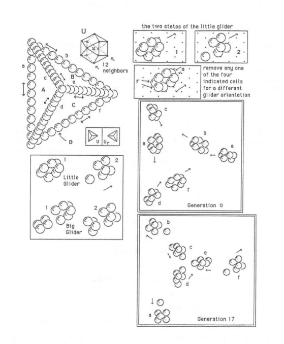
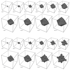
(Two examples of three-dimensional cellular automaton, Given in Stephen Wolfram’s A New Kind of Science)

     After further research, I found out some three-dimensional Game of Life. First we need to introduce a new naming method of  Game of Life.

      As we known, Conway’s Game of Life only has two  rules, one defines when to survive or die. The other one defines when to come alive. According to that, we can use a 4-tuple to define different Game of Life of different rules. Life ABCD means that (1) an alive cell survives when it touches at least A, at most B cell, it survive, otherwise it dies.(2) a dead cell comes to alive when it touches down to C, up to D cell. In this case, Conway’s Game of Life can be define as Life 2333.

      Carter Bays, in his paper “Candidates for the Game of Life in Three Dimensions”, defined that the naming method can only be used when following are True:

1.A glider must exist and must occur “naturally” if we apply repeatedly to primordial soup configurations.
2.All primordial soup configurations, when subjected to, must exhibit bounded growth.

      Carter Bays suggested that Life 4555 and Life 5766 are two best “worthy of the name” three-dimensional Game of Life. Thus, I turned to searched for some codes to test these two type of Life.

       3DGameofLife on GitHub is a JavaScript program created by Raphael Beaulieu and Elliot Coy. It can test three-dimensional Game of Life in a bounded space of 20×20×20. The complete code can be seen when we check the source code of the page, thus I am not going to paste it here. 

      First, going to test Life 4555. When I began the game with 7 cells of a 3D cross shape, The game showed a pattern of blinker. It stably iterates between three shape. 

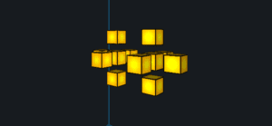
      Then, going to run Life 4555 again. This time, I began the game with 12 cells with the following shape.

      This time, even with the same rules, cells shows a totally different pattern. The number of cells explodes in a very short of time.

       Still, running Life 4555, with 5 cells of 2D cross shape. It turned out to be a third pattern. The cross repeatedly produced itself on the both way of the same line.

      Finally, testing the rule 5677. It showed a pattern of glider. The glider moved diagonally in one plane. However, it is worth to mention that the plane is parallel with one axis and  perpendicular to the other two axis, which means that the moving of the glider is kind of restricted.

Interestingly we can see that even under same rules, the outcomes will be significantly different because of the different input parameters, even when the differences between the input parameters are quite little. From my view, it is pretty similar to the beginning of life. Even there are planets other than Earth offer exactly same condition on Earth,  Our planets may be the only one holds the promise of life. 

Also, I find out that all the patterns under three-dimensional Game of Life I achieve above can actually acquired in the two-dimensional Game of Life. To some extend, it proves Bays’ saying “adding more dimensions does not ultimately seem to have much effect on the occurrence of behavior of any significant complexity”. However, since two-dimensional space is not visible, is that possible for two-dimensional creatures that we cannot  see existed as dimension seems not to be an important factors of complexity. That will be a left question for me.

Cite:

Candidates for the Game of Life in Three Dimensions’, Complex Systems, Carter Bays, Columbia, SC 29208, USA,

https://pdfs.semanticscholar.org/c865/e0d19f53ba646e076d6e542e1002c92fd3ad.pdf

Wolfram, Stephen. “Two Dimensions and Beyond”, A New Kind of Science, 1959, Wolfram Media

https://www.wolframscience.com/nks/chap-5–two-dimensions-and-beyond/

3DGameofLife, Raphael Beaulieu, Elliot Coy

http://rbeaulieu.github.io/3DGameOfLife/3DGameOfLife.html?

Lab Report: The Game of Life


Introduction:

The rule of “The Game of Life” in two dimension is defined on an infinite plane divided into a number of adjacent square, with each one surrounded by eight. Each square is considered as a “cell” with two attributes: Alive & dead, with the rules of altering between the to attributes shown below:

       If cell == alive {cell = dead if surrounded by n < 2 or n > 3 cells}; (living condition)

       If cell == dead {cell = alive if surrounded by n == 3 cells}; (reviving condition)

One “Generation” is defined as applying the two rules above simultaneously once. 

This report studies different algorithms which implement it, and how the rules behave on different two dimensional spaces through the algorithm.

Algorithm Analyzation:

1.  In two dimensional flat plane, the algorithm realizations is coded in  C#, which core part includes defining a three dimensional array to express a 100 x 100 2D plane and the correspondent cell value: 

private int[][] cellValues = new int[100][];

for (int r = 0; r < 99; r ++) {cellValue[r] = new int[100];}

using the “surrounding function” to tell how many other cells surround one, for example:

private int surrounding(int c, int v)
{if cellValue[r][c - 1] > 0 {count ++};}

Then it pass the count ‘g’ as the cell value to the correspondent cell value:

cellValue[r][c] = g;

To make one generation, the algorithm firstly calculate the cell value of every cell on the plane, then if a cell’s value is above 0, it will be activated, else it will be deactivated in the GUI codes.  

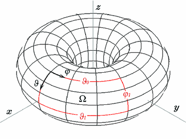
2. Another algorithm realized it in two dimensional toroidal surface via Python.

Enlarge

430402_1_En_3_Fig1_HTML
A toroidal surface

 The algorithm uses similar idea to tell whether a cell is alive or dead after one generation, that is, first calculate the cell value of every cell, then update the attribute of each. However, to express a toroidal surface in a regular two dimensional list: 

total = int((grid[i, (j - 1) % N] + grid[i, (j + 1) % N]
+ grid[( i - 1 ) % N,  j]+ grid[(i + 1) % N,  j]
 + grid[(i - 1) % N, (j - 1) % N] + grid[(i - 1) % N, (j + 1) % N]
+ grid[(i + 1) % N, (j - 1 ) % N] + grid[(i + 1) % N, (j + 1) % N])/255)

What’s special here is the mod operator (%), when a counting index goes out of the plain, it “drags” the index back. For example, in a 10 x 10 plane, the point (9, 9) connects to: (8, 9), (9, 8), (8, 8), (8, 0), (9, 0), (0, 0), (0, 9), (0, 8). Thus, if being observed on a 2D flat plane, a pattern will appear from another side of the plane if it reaches one boundary.

Rule Analyzation:

The report specially studies the reviving condition: why the conditional number is n = 3 but not others, using the Python code on toroidal surface.

The Python code provides several stable pattern on n = 3. Among them, A Glider is a small pattern moves diagonally, and a Gosper is a larger pattern that keeps firing Gilders. As they can represent the behavior of motion and reproduction, the report uses them as two study objects.

Enlarge

Rules_of_Conway%27s_game_of_life_-_Glider
A Glider

Enlarge

File:Gospers_glider_gun
A Gosper

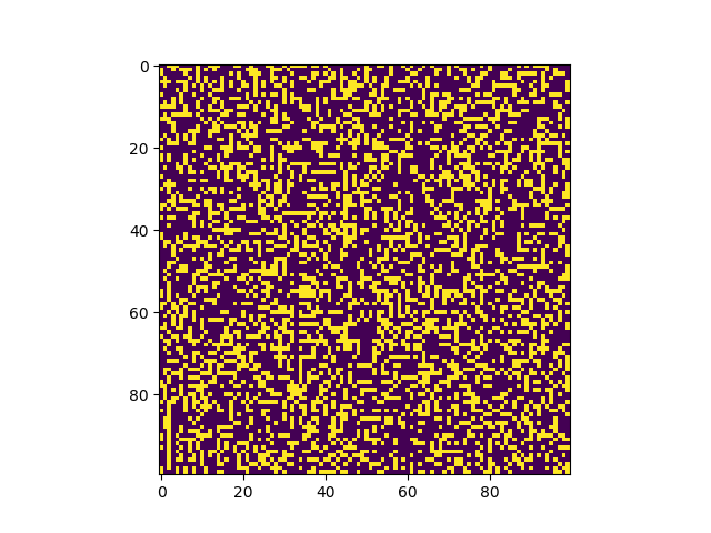
By experiment it shows when n = 4 or above the glider stays put without any motion and the Gosper ceased to a pairs of a-group-of-four blocks, which is a classic static pattern in Game of life. When n = 2, both patterns quickly expand and fill the whole surface with random moving patterns. Other experiments reveal similar results.

Enlarge

Figure_1
A chaotic pattern in n = 2

The experiment shows that it is reasonable to set the reviving condition to n = 3, as when n < 3 it is too easy for a cell to revive and the surface will be filled with chaotic moving patterns. and when n > 4 it is relatively difficult for cells to revive, thus the active patterns in n = 3 condition will be likely to stay stationary. n = 3 may be the rule for existing the most number of stable patterns.

However, further experiment find in n = 2, a flat plane is slower than a toroidal surface to become chaotic. Thus, it is likely that the reviving condition n is connected to the type of the space in order to create a rule with most stable patterns. For example, in 3D,4D Euclid space, or Rehman space the best reviving condition may not be 3. A correspondent function: best reviving condition = f(space type) may exist.

A study on 3D Euclid situation done by Carter Bays shows there are more cases in Game of Life on different spaces for further exploration.

Enlarge

捕获-1
A pattern in 3D space

Sources: 

MATHEMATICAL GAMES The fantastic combinations of John Conway’s new solitaire game “life”, by Martin Gardner, Scientific American 223 (October 1970): 120-123. https://web.stanford.edu/class/sts145/Library/life.pdf

Candidates for the Game of Life in Three Dimensions’, Complex Systems 1 (1987) 373-400, Carter Bays, Department of Computer Science, University of South Carolina, Columbia, SC 29208, USA, https://pdfs.semanticscholar.org/c865/e0d19f53ba646e076d6e542e1002c92fd3ad.pdf

C# code.
https://code.msdn.microsoft.com/windowsdesktop/Conways-Game-of-Life-75508f8f

Python code.  https://github.com/electronut/pp/blob/master/conway/conway.py 

Reflection # 3 – The Game of Life

Synopsis: This is an article from ‘The Guardian’ which using youtube videos gives an introduction to the mathematical recreation and its astounding patterns. The article ends with a video interview with the creator John Conway explaining his thought process when designing the rules.

In short Conway states that the beauty of Life is that it stands to reason that since you couldn’t predict what could happen ever, it is safe to say that anything can happen.

Questions: 

  • After reading The Crucial Experiment the value of this universe is a bit more apparent but still I have to question, what truly is its purpose?
  • Conway stated that the Game of Life came about from a desire to solve the challenge of creating a machine capable of building itself, while I don’t fully understand how Life solves this, it comes into question… can this be considered a rudimentary version of machine learning?
  • If there are rules but the patterns are unpredictable what do the rules prove? 
    • It almost works like some sort of negative induction or null hypothesis
  • A follow up to the previous question would be are there finite sets of rules that don’t develop into a regulated pattern?

Reflection #2 – The Crucial Experiment

Synopsis: This reading was an except from Stephen Wolfram’s The Crucial Experiment – A New Kind of Science. The except looked at cellular automata* and asked the question “Can Complexity come from Simplicity?” 

Questions: 

  • My biggest question for this reading was, why is this information useful? 
  • What is the different between one dimensional (Game of Life)  and two dimensional (cellular automata)?
  • Why the fundamental idea that nature works like these complex automata in that it all stems from simple beginnings, how can actual rules and examples help us better understand nature.
  • How are these autonomous agents programmed (purpose of the lab I assume)
  • Does a step refer to a change in a cell or a change in a row.

Notes:

  • Cellular Automata is easy to follow since their behaviour must have the ability to be readily presented in a visual way.
  • Fractal Patterns are the perfect balance between complexity and simple repetition
  • The basic phenomenon is ultimately responsible for most of the complexity in nature
  • Even though cells follow the same rules, different configurations of cells will have different behaviour

Thoughts on Lab:

  • Physical computation behaves similarly to cellular automation
    • executing few simple instructions in large numbers generating complexity
    • however this is just one aspect of computation
    • understanding how to generate autonomous agents on through cellular automata, we can apply skills to creating autonomous robots which is basically the foundation of nature’s complexity 

Cellular Automata is a collection of “coloured” cells on a grid of specified shape that evolves through a number of discrete time steps according to a set of rules based on the states of the neighbouring cells. Rules are then applied iteratively for as many steps as desired.