Idea:
For a long time, I was interested in exploring the possible connections between facial expression, presentation and personality. The topic of biological determinism and the degree to which it can accurately describe the complexity of personality traits has long been a topic of a racially and politically charged discourse. The project presented below is an exploration in possibilities and limitations of such modelling, as well as an attempt to bring back right to self-reflection and self-determination to the person who is being watched.
Background:
The alleged connection between shape of human head and innate traits has been quite contentious, but this did not prevent certain ideologies to make use of its “scientific” appeal. In the 19th century, the pseudoscience of character reading named phrenology has gained enormous popularity in the Anglo – Saxon countries, particularly the United States. The growth in popularity has been engendered by the relatively recent hypothesis that the brain was the “organ of the mind”, which eventually turned out to be true – just not in the ways phrenologists would like.
As proponents of the science imagined, the brain was an organ divided into separate sections, each responsible for different kind of variance in the mental faculty. However, the evidence provided was largely derived from confirmation seeking, with little effort to account for contradictory data. Scientification of racism (the “savage”-type brain), gender and class divisions (“highbrow” vs “lowbrow” distinctions) have for decades reinforced what would otherwise stay in the domain of social conditioning, therefore in the domain of social change.
In this way, it is somewhat similar to the research being done right now in terms of personality prediction
In the areas of AI and machine intelligence, there are several startups and research groups that specialise in determining personalities from historical facial data. One of them, Faception, is claiming to have found a way to determine potential terrorists from facial data. The models developed and presented are clearly ridden with racist bias. The way most of machine learning works is through learning from historical data, which is often loaded with bias, and then making future predictions based on it. In short: no matter how “intelligent” the model is, the “garbage in, garbage out” rule still applies.
The process:
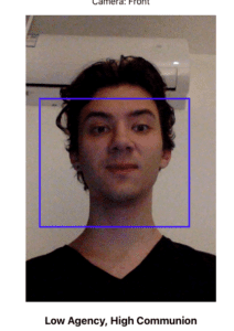
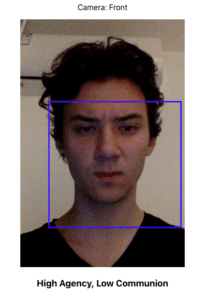
In the project, I decided to look into two specific traits: agency (defined as assertiveness and goal-orientedness) and communion (willingness to collaborate and socialise). These constitute the Big Two, which was most easy to infer.

The model is based off of a Basel Face Dataset, with labelled photos of 40 participants (50:50 gender breakdown), from whom photos have been taken and digitally altered to show variance in perceived personality. Although the dataset is relatively small, valid inferences can be made due to the fact that all samples have been validated by human subjects. Respondents have been hired through Amazon MTurk, who after being presented with photos, have answered questions about their response to the stimuli.
Due to the valid privacy concerns, it took me a week to gain access to the dataset. I had to send a request to the University of Basel, which then had to be cross-checked with the professor.
Having gained access, I started the initial exploration. It turned out that much of the variance in the faces can be found in bone structure. I looked at the photos and saw that individuals with low perceived agency have much less “sharp” facial features, which is especially visible on their eyebrows.
Therefore, I decided to use landmark detection for facial inferences. This has been generated with the OpenCV library. Then, I generated number-based labels for the personality data. It has not been generated by me. The files were labelled in the dataset, but only through their filenames and numbers. Therefore, I had to convert them into their numeric representations, ranging from 0 to 2.
Code for processing the data:
import cv2
import numpy as np
import dlib
import sys
import glob
import csv
imgs = []
path = “data/samples”
valid_images = [“.jpg”,”.gif”,”.png”,”.tga”]
detector = dlib.get_frontal_face_detector()
predictor = dlib.shape_predictor(“shape_predictor_68_face_landmarks.dat”)
landmarks_mx = []
filenames = glob.glob(“data/big_two/*.png”)
filenames.sort()
images = [cv2.imread(img) for img in filenames]
counter = 0
for image in images:
gray = cv2.cvtColor(image, cv2.COLOR_BGR2GRAY)
faces = detector(gray)
landmarks_row = []
for face in faces:
landmarks = predictor(gray, face)
landmarks_values = []
for n in range(0, 68):
x = landmarks.part(n).x
y = landmarks.part(n).y
cv2.circle(image, (x, y), 2, (255, 255, 255), -1)
landmarks_values.append(x)
landmarks_values.append(y)
if (0 == (counter % 4)):
landmarks_values.append(2)
landmarks_values.append(1)
elif (1 == (counter % 4)):
landmarks_values.append(0)
landmarks_values.append(1)
elif (2 == (counter % 4)):
landmarks_values.append(1)
landmarks_values.append(2)
elif (3 == (counter % 4)):
landmarks_values.append(1)
landmarks_values.append(0)
landmarks_row.append(landmarks_values)
counter += 1
landmarks_mx.append(landmarks_row)
with open(‘landmarks_file_big_two.csv’, mode=’w’) as landmarks_file:
landmarks_writer = csv.writer(landmarks_file, delimiter=’,’, quotechar='”‘, quoting=csv.QUOTE_MINIMAL)
for row in landmarks_mx:
landmarks_writer.writerow(row)
Training:
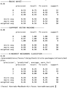
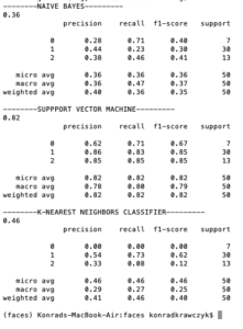
I trained the dataset using the TensorFlow neural network, and the results were very underwhelming. Therefore, I decided to immediately switch to an open-source tool that I have used in the past, namely sklearn. There, I used models that I thought would work better with the relatively small amount of data that I got access to. Surprisingly, support vector machine has worked very well, both in agency prediction (left) and communion prediction (right).
Code for the training phase
import array as arr
import numpy as np
import os
import csv
from sklearn.preprocessing import StandardScaler
from sklearn.preprocessing import Normalizer
from sklearn.model_selection import train_test_split
from sklearn.linear_model import LinearRegression
from sklearn.svm import SVC
from sklearn.naive_bayes import GaussianNB
from sklearn import neighbors
from sklearn.metrics import accuracy_score
from sklearn.metrics import classification_report
from sklearn.externals import joblib
batch_size = 32
num_classes = 10
epochs = 100
num_predictions = 20
class_names = [[‘Dominant’, ‘Submissive/Dominant’, ‘Submissive’ ], [‘Trustworthy’, ‘Somewhat Trustworthy’, ‘Untrustworthy’]]
big_two = []
originals = []
all_data = []
#convert the csv strings to a nice data matrix (Big Two)
with open(‘landmarks_file_big_two.csv’) as csv_file:
csv_reader = csv.reader(csv_file, delimiter=’,’, quotechar='”‘, quoting=csv.QUOTE_MINIMAL)
for row in csv_reader:
rowArr = list(map(int,row[0].replace(‘[‘, ”).replace(‘]’, ”).split(‘,’))) #map = to convert the number from string (some has also space ) to integer
big_two.append(rowArr)
with open(‘landmarks_file_originals.csv’) as csv_file:
csv_reader = csv.reader(csv_file, delimiter=’,’, quotechar='”‘, quoting=csv.QUOTE_MINIMAL)
for row in csv_reader:
rowArr = list(map(int,row[0].replace(‘[‘, ”).replace(‘]’, ”).split(‘,’))) #map = to convert the number from string (some has also space ) to integer
originals.append(rowArr)
#merge originals and big two data
all_data = big_two
i = 4
j = 0
while i <= len(big_two):
all_data.insert(i, originals[j])
i += 5
j += 1
#Prepare data for training
X = []
y = []
for row in all_data:
X.append(row[:-2])
#y.append(row[-2:-1])
y.append(row[-1:])
print(len(X))
print(len(y))
X = np.array(X)
y = np.array(y)
print(len(y))
X_train, X_test, y_train, y_test = train_test_split(X,y.ravel(),random_state=0)
# scaler = StandardScaler().fit(X_train)
# standardized_X = scaler.transform(X_train)
# standardized_X_test = scaler.transform(X_test)
#NAIVE BAYES
print(“——–NAIVE BAYES———“)
gnb = GaussianNB()
gnb.fit(X_train, y_train)
y_pred = gnb.predict(X_test)
gnb.score(X_test, y_test)
print(accuracy_score(y_test, y_pred))
print(classification_report(y_test, y_pred))
#SVM
print(“——–SUPPPORT VECTOR MACHINE———“)
svc = SVC(kernel=’linear’)
svc.fit(X_train, y_train)
y_pred = svc.predict(X_test)
svc.score(X_test, y_test)
print(accuracy_score(y_test, y_pred))
print(classification_report(y_test, y_pred))
#this is rly good save it as a pickle file
#joblib.dump(svc, ‘saved_model_communion.pkl’)
#KNN
print(“——–K-NEAREST NEIGHBORS CLASSIFIER———“)
knn = neighbors.KNeighborsClassifier(n_neighbors=5)
knn.fit(X_train, y_train)
y_pred = knn.predict(X_test)
knn.score(X_test, y_test)
print(accuracy_score(y_test, y_pred))
print(classification_report(y_test, y_pred))
Later I saved the model into a .pkl file, and rolled out an API using flask. (Repo available here https://github.com/krawc/faces-restful).
Then, I developed a front-end tool, which has been the most difficult part.
This is the version after refinement and style fixes. It still takes a considerable amount of time to load the model, so it might work at the second try only (depending on the connection speed)


Repo: https://github.com/krawc/faces-frontend
Demo: https://faces-frontend.herokuapp.com/
Reflection:
The tool I developed has a surprising accuracy, for the relatively small amount of unprocessed data that has been used. After having tested it, I can see that the patterns from photos are reflected in the common usage of the app. What I am most interested in, however, is how this can be related to the users’ perceptions of themselves. If I can measure how accurate a model is for “perceived” personality, it is also important to measure how this perception relates to reality, or whether at all. The interactive part could also be further developed, and design could be improved.