The final exam for the Fall 2017 Numerical Methods class consisted in performing a project. Each student had to study some additional theory and write a code to numerically solve a mathematical problem.
The depth, breadth and quality of their work is outstanding! Here’s a brief summary of what they did.
- Titas Geryba: Nonlinear differential algorithm to compute all the zeros of a generic polynomial.
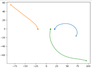
A recent paper by prof. Francesco Calogero shows that the zeros of a polynomial may be found by solving a certain system of nonlinear differential equations involving the polynomial’s coefficients. For polynomials of arbitrary order the solutions can’t be found with paper and pen, therefore numerical methods must be used. The following figure shows the solutions in the complex plane of these ODEs for the polynomial \(P(z)=(z-20)(z+20)(z-10)\). Starting from arbitrary initial conditions, the solutions at time t=1 approximate the zeros. These approximations may be taken as new initial conditions, and the solution process may be iterated a few times in order to achieve a very high accuracy. - Ziyuan (Jennifer) Huang: Simulations of a bouncing rod.
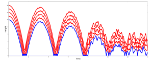
A rod of elastic material bouncing vertically over a rigid floor is simulated as a chain of point masses connected by linear, dissipationless springs. Each time that the lowest point mass hits the floor its velocity reverses. The simulation illustrates the transfer of potential gravitational energy into energy of the vibrational modes. - Frederik Jensen: Liquidity Reserve Control.
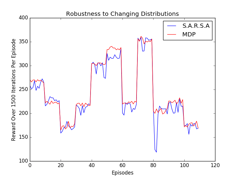
The need for a currency broker to maintain her reserves liquid is vital to business. If the broker runs low on any reserve, possible consequences range from increased commission rates, a cap on withdrawal, or discontinuement of supply until the reserve has been replenished. This projects aims at building a revenue maximising solution for strongly competitive brokers by casting the liquidity issue as a control problem and adopting a reinforcement learning approach. In particular, the scope of the problem considered extends to brokers that deal with cryptocurrencies as well. - Myera Rashid: Pattern formation in the FitzHugh-Nagumo equations.
The foundations for a mathematical understanding of pattern formation in biological systems were laid down by Alan Turing (yes, that Turing) in a seminal paper. An example of pattern-forming equations is obtained by adding diffusion terms to the FitzHugh-Nagumo equations. The movie shows the early phases of pattern formation, starting from random initial conditions, on a doubly-periodic domain with 50×50 grid nodes. An explicit FTCS scheme is used to numerically solve the equations. - Jin Shang: A simple model of traffic flow.
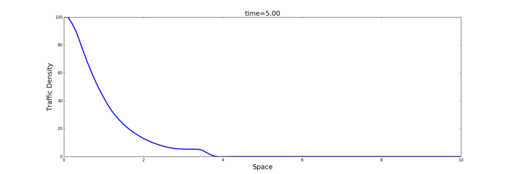
An important topic in civil engineering is modelling the flow of cars along roads. The earliest model, due to Lighthill and Whitham captures a wide variety of traffic flow phenomena in a surprisingly simple conservation law. The following figure shows a rarefaction wave of a long queue of cars some time after a street light has become green. - Boyan Stoychev: Solving PDEs via pseudospectral methods.
Pseudospectral methods are a class of powerful numerical methods for solving PDEs in simple domains. In this project a simple Galerkin method is used to numerically solve Burger’s equation and Schrödinger’s equation with a variety of potentials. The following movie shows the modulus of the wavefunction of a Gaussian wavepacket (blue) impinging on a very tall potential barrier (black). In classical mechanics a particle with the same energy of the wavepacket could not pass the barrier. In quantum mechanics, if the barrier is sufficiently thin, there is a non–negligible probability to find the particle on the other side of the barrier, signaled by the splitting of the wavefunction in two (roughly Gaussian) parts. - Silviu Udrescu: Three bodies restricted problem and symplectic integrators.
Some ODEs have a special structure, known as symplectic. The most notable application that gives rise to such ODEs is Hamiltonian classical mechanics. Standard numerical integrators do not respect the symplectic structure of ODEs, giving rise to subtle errors (diagnosable by a lack of conservation of energy) that pile up in long integrations, until the result becomes unusable. Symplectic integrators are numerical methods that approximate a symplectic ODE with a symplectic map, thereby imposing conservation properties as close as possible to those of he original equations. The following animation shows the chaotic orbit of a tiny planet in a binary stellar system (it’s called the restricted three-body problem) integrated through a sixth-order, symplectic Runge-Kutta method. - Alexandra Urbanikova: Numerical analysis of bifurcations.
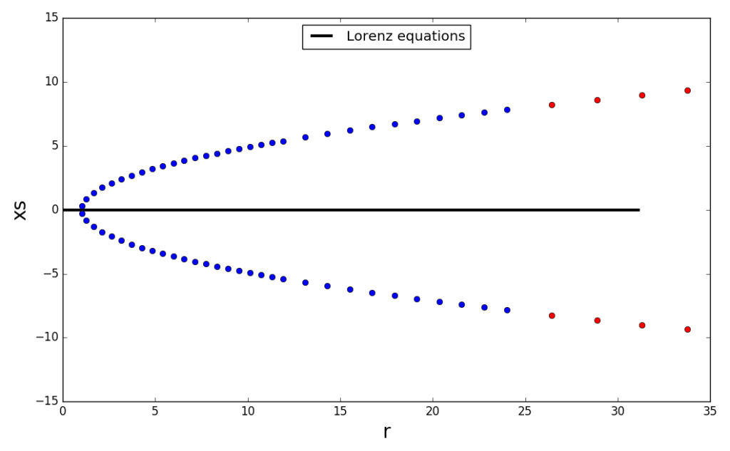
Upon changing the numerical value of a parameter in an ODE, the number and stability of equilibria may change. When this occurs, it is said that the system has undergone a bifurcation. A numerical continuation code is able, as the parameter changes, to follow the position of the equilibria and detect bifurcations by monitoring stability changes. The following figure shows an example of numerical continuation for the celebrated Lorenz system. - Sunyi Wang: Simulations of shallow wave equations in 1D.
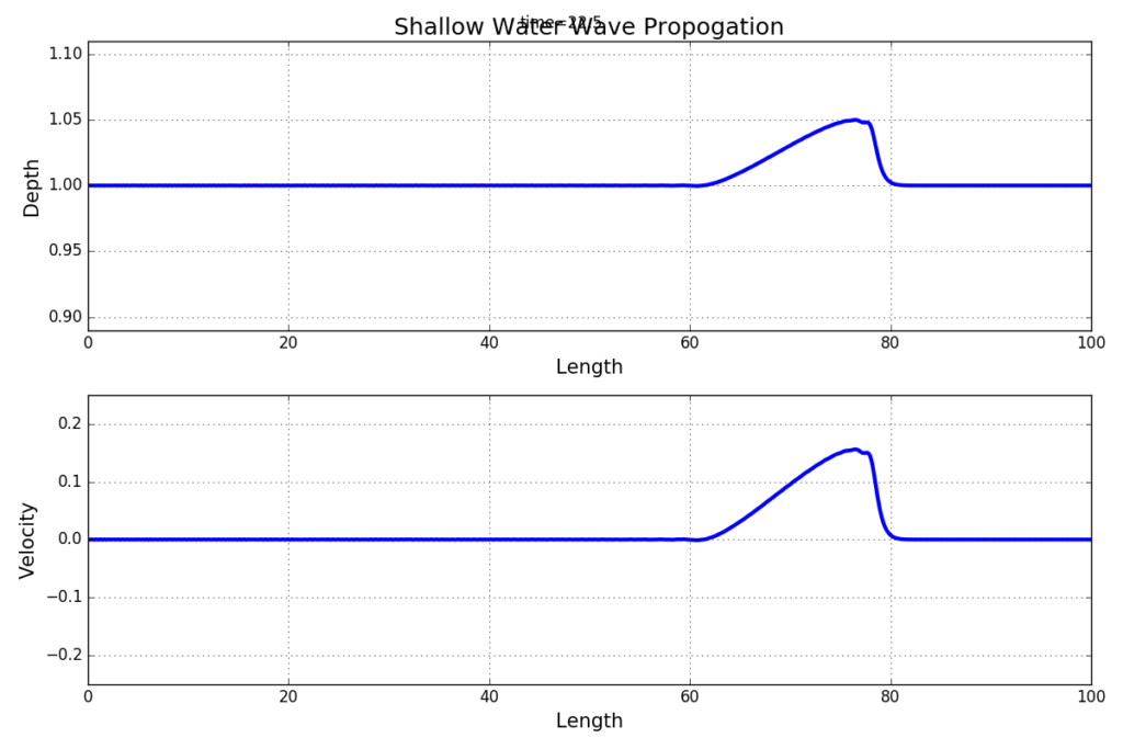
Shallow wave equations describe thin layers of fluid with a free surface. They have strong similarities with compressible flows. In the following figure it is shown a nonlinear wave that evolved from an initially sinusoidal bump. - Lin Zhu: Numerical solution of 2D Navier-Stokes equations.
Incompressible fluid motions require the solution of an elliptic problem to be numerically computed. In 2D, when one uses the streamfunction-vorticity formulation (which is convenient to avoid dealing with pressure), to this difficulty one must add that simple centered finite differences methods tend to be unstable. An elegant fix is to use Arakawa’s discretization of the Jacobian. The following animation shows the evolution of vorticity starting from a symmetric initial condition.

