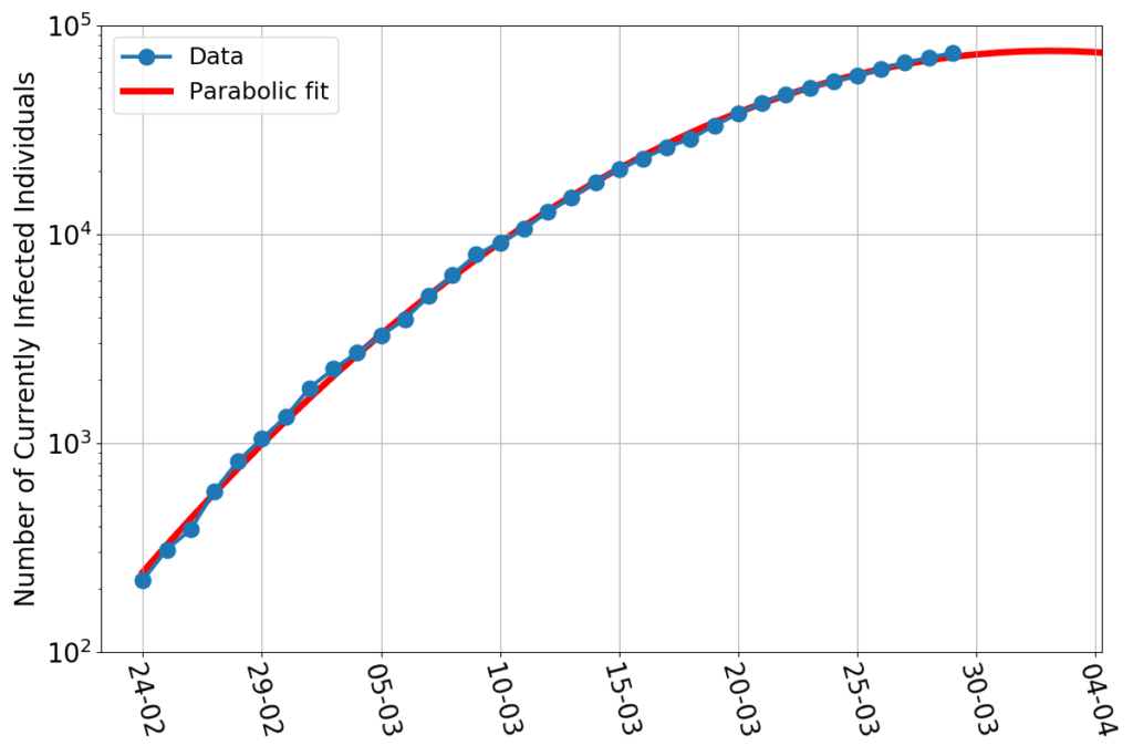
Today’s data look this way:

On a vertical axis logarithmic scale the data points still nicely align along a parabolic fit. The maximum of this fit, however, didn’t stay put. It now has shifted to about April 2nd, and the last few points are a little above the curve, so it’s quite likely to keep shifting in the next few days. 

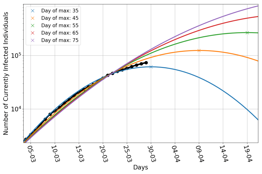
There’s news, however. If I repeat the exercise of fitting parabolas whose maximum is set beforehand, (see here for details), I now find this:

The data points appear to be wedged between the parabola peaking on March 30th and that peaking on April 9th. Shifting the peak much beyond that date would require a significant deviation from the parabolic trend.

Big deal! – One might say. After all, there’s no obvious theoretical reason to believe that the data have to align along a parabolic trend. If no natural law forces them to take that shape, then we shouldn’t hope to see them following that pattern forever. And yet, so far, they did. 

This calls for a little additional investigation.

I said that the number of currently infected individuals $I$, seen as a function of time, must obey the equation $$\frac{dI}{dt}=r(t) I$$ (last time I used Newton’s dot notation $\dot{I}$ for the time derivative of $I$). This is always true, provided that one picks the correct growth rate function $r$. And this, obviously, begs the question of who or what is going to tell us which is such an $r$. Well, the honest answer is: no one. But thinking in terms of growth rate, rather than in terms of number of infected individuals, may give us a more powerful (albeit more abstract) way to think about the epidemics.

If you have ever taken calculus, you’ll now that the equation can be rearranged in this way: $$\frac{d \log(I)}{dt} = r(t).$$ In plain English, this tells us that the rate of change of the logarithm of $I$ is the same thing as the growth rate. 

If one plots a function (say, the number of currently infected individuals vs time) using a logarithmic scale on the vertical axis, that’s obviously just the same as plotting the logarithm of the same function on regular axes. 

So, the above equation tells us that, at each time $t$, the growth rate is just the slope of the curve that we see in the first figure of this post. As you might recall from calculus, if you were to draw the values of slopes at each point along a parabola, you’d get a straight line.

In short, and in the simplest possible terms: if the infection shows a parabolic trend on a log-scale graph, then its growth rate decreases linearly in time. The converse is also true; if the growth rate decreases linearly, then the trend of the infection will be parabolic (on a log-scale graph).

So, on one hand we should really look at the growth rate, and see if it goes straight, on the other hand, the growth rate is the one thing that we don’t know.

Ouch! 

Well, we still have the data. And we can use them to compute some approximate estimate of the true growth rate. I shall use the simplest and crudest one: $$r(n) \approx \frac{I(n)-I(n-1)}{I(n)}.$$ That is, the growth rate at day $n$ is the ratio between the increment of infected with respect to day $n-1$ and the total number of infected at day $n$.

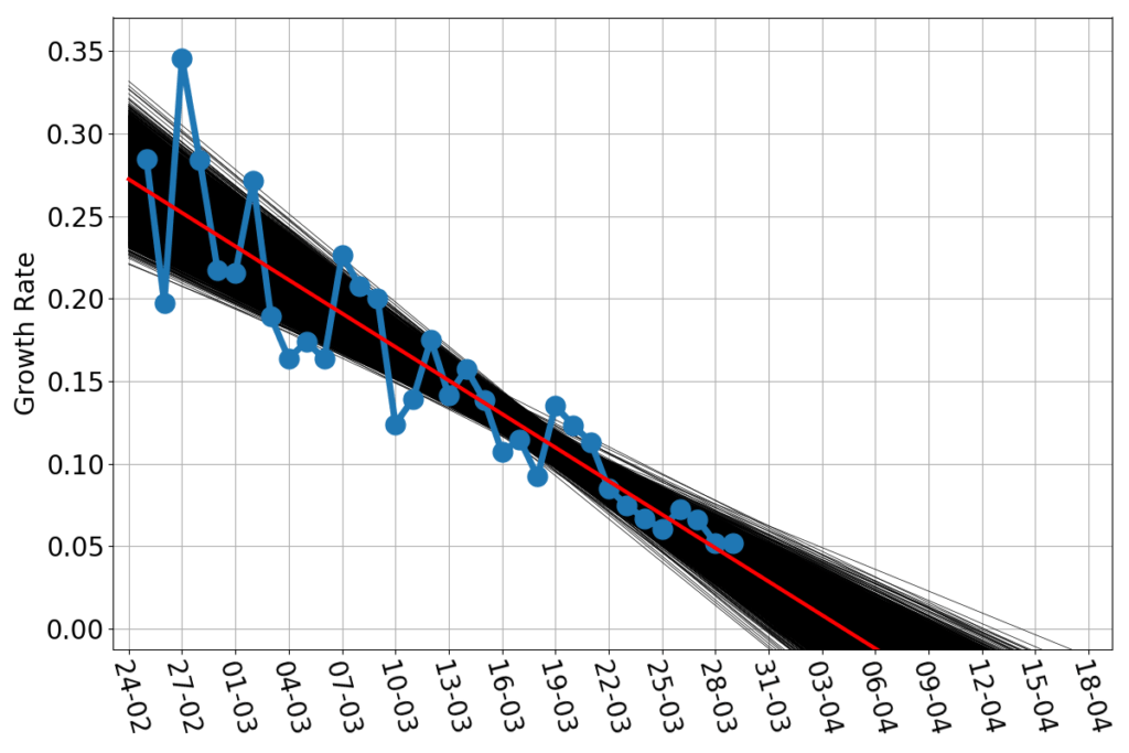
This yields the blue dots in the following figure:

The estimated growth rate wiggles a lot, in particular in the early part of the time series, but surely seems to have a downward linear trend. The red line is the straight line that best fits the blue dots. As before, we should note that the best fit is not the only reasonable fit. What would be the variation among fitting lines that are decent approximations to the data? The answer obviously depends on what is your criterion for a “decent” fit, as well as a host of other hypothesis. I’ll just go the rough and easy way: bootstrapping my data set.  Imagine to put your $m$ data points in a jar, extract one, note what that is, reinsert it into the jar. Shake the jar and repeat $m$ times. Now, on your notes, you have a new dataset of $m$ data points. Most likely, some of them are repeated (they’ve been extracted twice or more), and some that appeared in the original dataset are missing (they’ve never been extracted). And yet the straight line which is the best fit for such a bootstrapped dataset is also a decent fit for the original one. The beauty of bootstrapped datasets is that, even with few data points, there’s plentiful. The 10000 black lines in the above figures are each the best fit to 10000 bootstrapped versions of the blue data points. That bunch of black lines shows visually how much, at most, we can expect the red line to be wrong. Provided, of course, that the growth rate really keeps a linear trend.

I don’t think it will. Maybe it’s the late hour, maybe it’s the long days of home confinement, but I’m not so inclined to optimism. It appears that the public health measures have slowly, steadily decreased the growth rate of the epidemics. But can they bring it to a halt, and then make it negative? 

That’s the topic for another post.

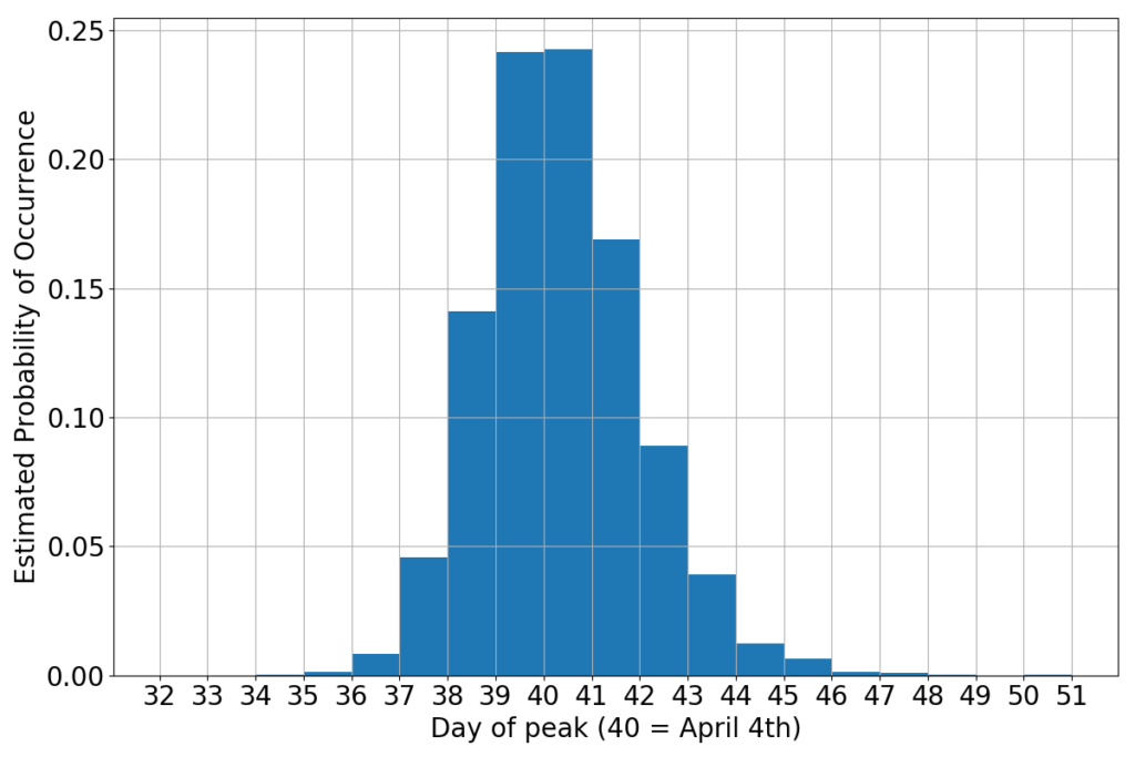
For now, I just say that if the growth rate really decreases in time as a straight line, then we have another predictor for the peak. The peak, obviously, is the moment when the infection curve will neither grow, nor decrease. That’s growth rate zero. We now have ten thousand different estimates for such a zero (one for each black line). All together they yield this probability curve:

 

If you believe this little alchemy (the math is sound, but the hypothesis that the growth rate will keep straight is a gamble) then the peak should occur sometimes during the first week of April. Not surprisingly, this is consistent with the wedging of the data between the parabola peaking on March 30th and that peaking on March 9th. It’s just a different way to say the same thing.

It wouldn’t be bad if it stayed this way…